Article Structure
Abstract
Counts from large corpora (like the web) can be powerful syntactic cues.
Introduction
Current state-of-the art syntactic parsers have achieved accuracies in the range of 90% F1 on the Penn Treebank, but a range of errors remain.
Web-count Features
Structural errors in the output of state-of-the-art parsers, constituent or dependency, can be viewed as attachment errors, examples of which are Figure 1 and Figure 2.1 One way to address attachment errors is through features which factor over head-argument
Working with Web n-Grams
Previous approaches have generally used search engines to collect count statistics (Lapata and Keller, 2004; Nakov and Hearst, 2005b; Nakov and Hearst, 2008).
Parsing Experiments
Our features are designed to be used in full-sentence parsing rather than for limited decisions about isolated ambiguities.
Analysis
Table 4 shows error counts and relative reductions that our web features provide over the 2nd-order dependency baseline.
Conclusion
Web features are a way to bring evidence from a large unlabeled corpus to bear on hard disambiguation decisions that are not easily resolvable based on limited parser training data.
Topics
n-grams
- Instead, we consider how to efficiently mine the Google n-grams corpus.Page 2, “Introduction”
- This work uses a large web-scale corpus (Google n-grams ) to compute features for the full parsing task.Page 2, “Introduction”
- The approach of Lauer (1995), for example, would be to take an ambiguous noun sequence like hydrogen ion exchange and compare the various counts (or associated conditional probabilities) of n-grams like hydrogen ion and hydrogen exchange.Page 3, “Web-count Features”
- (2010) use web-scale n-grams to compute similar association statistics for longer sequences of nouns.Page 3, “Web-count Features”
- These paraphrase features hint at the correct attachment decision by looking for web n-grams with special contexts that reveal syntax superficially.Page 4, “Web-count Features”
- We take each (correct) training dependency relation (h, a) and consider web n-grams of the form cha, hca, and hac.Page 4, “Web-count Features”
- For example, for h = raising and a = from (see Figure l), we look at web n-grams of the form raising c from and see that one of the most frequent values of c on the web turns out to be the word it.Page 4, “Web-count Features”
- Rather than working through a search API (or scraper), we use an offline web corpus — the Google n-gram corpus (Brants and Franz, 2006) — which contains English n-grams (n = l to 5) and their observed frequency counts, generated from nearly 1 trillion word tokens and 95 billion sentences.Page 4, “Working with Web n-Grams”
- In particular, we only use counts of n-grams of the form :3 * y where the gap length is g 3.Page 4, “Working with Web n-Grams”
- Next, we exploit a simple but efficient trie-based hashing algorithm to efficiently answer all of them in one pass over the n-grams corpus.Page 5, “Working with Web n-Grams”
- With this representation of our collection of queries, we go through the web n-grams (n = 2 to 5) one by one.Page 5, “Working with Web n-Grams”
See all papers in Proc. ACL 2011 that mention n-grams.
See all papers in Proc. ACL that mention n-grams.
Back to top.
dependency parsing
- We show relative error reductions of 7.0% over the second-order dependency parser of McDonald and Pereira (2006), 9.2% over the constituent parser of Petrov et al.Page 1, “Abstract”
- For dependency parsing , we augment the features in the second-order parser of McDonald and Pereira (2006).Page 2, “Introduction”
- (2008) smooth the sparseness of lexical features in a discriminative dependency parser by using cluster-based word-senses as intermediate abstractions inPage 2, “Introduction”
- For the dependency case, we can integrate them into the dynamic programming of a base parser; we use the discriminatively-trained MST dependency parser (McDonald et al., 2005; McDonald and Pereira, 2006).Page 2, “Introduction”
- pairs, as is standard in the dependency parsing literature (see Figure 3).Page 3, “Web-count Features”
- We first integrate our features into a dependency parser , where the integration is more natural and pushes all the way into the underlying dynamic program.Page 5, “Parsing Experiments”
- 4.1 Dependency ParsingPage 5, “Parsing Experiments”
- For dependency parsing , we use the discriminatively-trained MSTParser4, an implementation of first and second order MST parsing models of McDonald et a1.Page 5, “Parsing Experiments”
- Table 1: UAS results for English WSJ dependency parsing .Page 6, “Parsing Experiments”
- (2009), K00 and Collins (2010) has been exploring more nonlocal features for dependency parsing .Page 6, “Parsing Experiments”
- Results are for dependency parsing on the dev set for iters:5,training-k:1.Page 7, “Analysis”
See all papers in Proc. ACL 2011 that mention dependency parsing.
See all papers in Proc. ACL that mention dependency parsing.
Back to top.
Berkeley parser
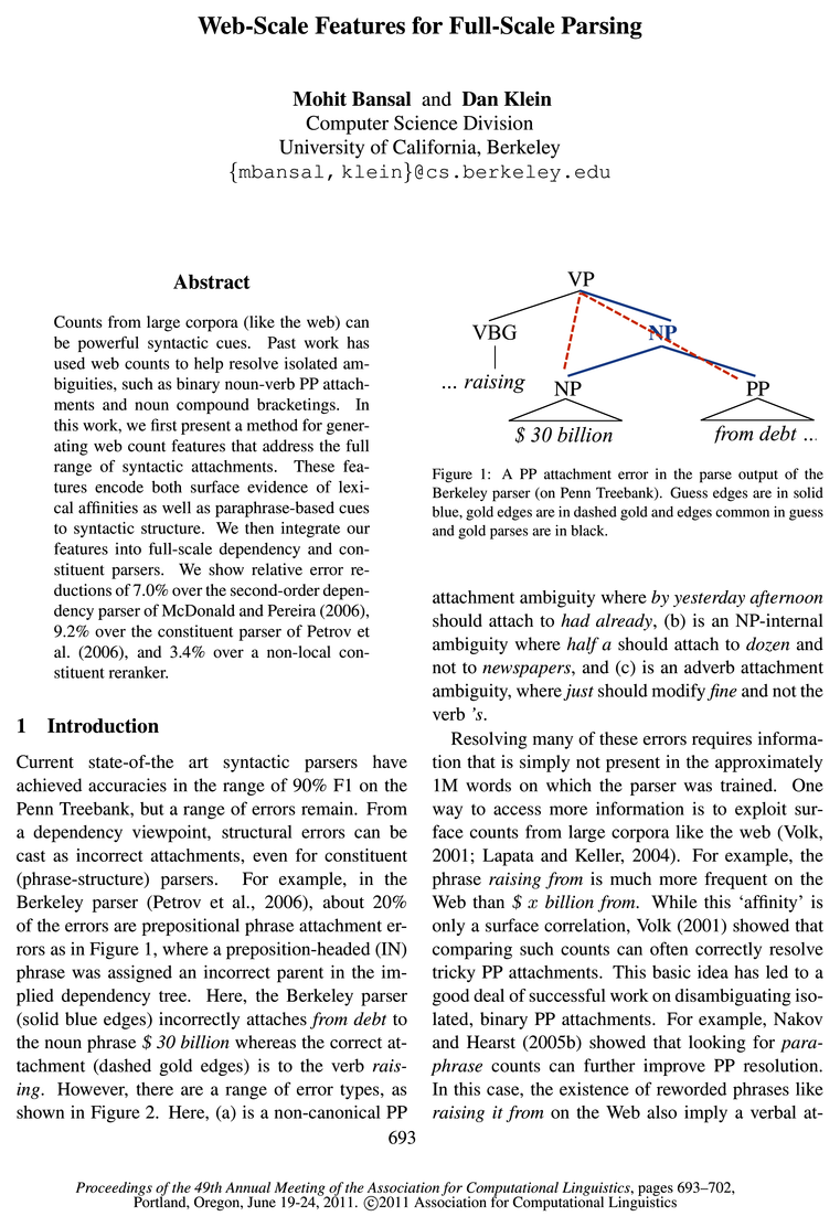
- For example, in the Berkeley parser (Petrov et al., 2006), about 20% of the errors are prepositional phrase attachment errors as in Figure l, where a preposition-headed (IN) phrase was assigned an incorrect parent in the implied dependency tree.Page 1, “Introduction”
- Here, the Berkeley parser (solid blue edges) incorrectly attaches from debt to the noun phrase $ 30 billion whereas the correct attachment (dashed gold edges) is to the verb raising.Page 1, “Introduction”
- Figure l: A PP attachment error in the parse output of the Berkeley parser (on Penn Treebank).Page 1, “Introduction”
- For constituent parsing, we rerank the output of the Berkeley parser (Petrov et al., 2006).Page 2, “Introduction”
- For constituent parsing, we use a reranking framework (Charniak and Johnson, 2005; Collins and Koo, 2005; Collins, 2000) and show 9.2% relative error reduction over the Berkeley parser baseline.Page 2, “Introduction”
- We also evaluate the utility of web-scale features on top of a state-of—the-art constituent parser — the Berkeley parser (Petrov et al., 2006), an unlexical-ized phrase-structure parser.Page 6, “Parsing Experiments”
- Our baseline system is the Berkeley parser , from which we obtain k-best lists for the development set (WSJ section 22) and test set (WSJ section 23) using a grammar trained on all the training data (WSJ sections 2-21).8 To get k-best lists for the training set, we use 3-fold jackknifing where we train a grammarPage 6, “Parsing Experiments”
- Table 2: Oracle Fl-scores for kr-best lists output by Berkeley parser for English WSJ parsing (Dev is section 22 and Test is section 23, all lengths).Page 6, “Parsing Experiments”
- 9Default: we ran the Berkeley parser in its default ‘fast’ mode; the output kr-best lists are ordered by max-rule-score.Page 6, “Analysis”
- Table 3: Parsing results for reranking 50-best lists of Berkeley parser (Dev is WSJ section 22 and Test is WSJ section 23, all lengths).Page 7, “Analysis”
See all papers in Proc. ACL 2011 that mention Berkeley parser.
See all papers in Proc. ACL that mention Berkeley parser.
Back to top.
constituent parser
- We then integrate our features into full-scale dependency and constituent parsers .Page 1, “Abstract”
- We show relative error reductions of 7.0% over the second-order dependency parser of McDonald and Pereira (2006), 9.2% over the constituent parser of Petrov et al.Page 1, “Abstract”
- For constituent parsing , we rerank the output of the Berkeley parser (Petrov et al., 2006).Page 2, “Introduction”
- To show end-to-end effectiveness, we incorporate our features into state-of-the-art dependency and constituent parsers .Page 2, “Introduction”
- For constituent parsing , we use a reranking framework (Charniak and Johnson, 2005; Collins and Koo, 2005; Collins, 2000) and show 9.2% relative error reduction over the Berkeley parser baseline.Page 2, “Introduction”
- 1For constituent parsers , there can be minor tree variations which can result in the same set of induced dependencies, but these are rare in comparison.Page 2, “Web-count Features”
- We then add them to a constituent parser in a reranking approach.Page 5, “Parsing Experiments”
- 4.2 Constituent ParsingPage 6, “Parsing Experiments”
- We also evaluate the utility of web-scale features on top of a state-of—the-art constituent parser — the Berkeley parser (Petrov et al., 2006), an unlexical-ized phrase-structure parser.Page 6, “Parsing Experiments”
- We next investigate the features that were given high weight by our learning algorithm (in the constituent parsing case).Page 7, “Analysis”
See all papers in Proc. ACL 2011 that mention constituent parser.
See all papers in Proc. ACL that mention constituent parser.
Back to top.
reranking
- (2006), and 3.4% over a nonlocal constituent reranker .Page 1, “Abstract”
- For constituent parsing, we rerank the output of the Berkeley parser (Petrov et al., 2006).Page 2, “Introduction”
- For constituent parsing, we use a reranking framework (Charniak and Johnson, 2005; Collins and Koo, 2005; Collins, 2000) and show 9.2% relative error reduction over the Berkeley parser baseline.Page 2, “Introduction”
- We then add them to a constituent parser in a reranking approach.Page 5, “Parsing Experiments”
- We also verify that our features contribute on top of standard reranking features.3Page 5, “Parsing Experiments”
- Because the underlying parser does not factor along lexical attachments, we instead adopt the discriminative reranking framework, where we generate the top-k candidates from the baseline system and then rerank this k-best list using (generally nonlocal) features.Page 6, “Parsing Experiments”
- Next, we rerank with only the features (both local and nonlocal) from Huang (2008), a simplified merge of Charniak and Johnson (2005) and Collins (2000) (here configurational).Page 6, “Parsing Experiments”
- Finally, we rerank with both our Web-scale features and the configurational features.Page 6, “Parsing Experiments”
- When combined, our web-scale features give a further error reduction of 3.4% over the configurational reranker (and a combined error reduction of 12.2%).Page 6, “Parsing Experiments”
- Table 3: Parsing results for reranking 50-best lists of Berkeley parser (Dev is WSJ section 22 and Test is WSJ section 23, all lengths).Page 7, “Analysis”
See all papers in Proc. ACL 2011 that mention reranking.
See all papers in Proc. ACL that mention reranking.
Back to top.
n-gram
- (2010), which use Web-scale n-gram counts for multi-way noun bracketing decisions, though that work considers only sequences of nouns and uses only affinity-based web features.Page 2, “Introduction”
- Lapata and Keller (2004) uses the number of page hits as the web-count of the queried n-gram (which is problematic according to Kilgarriff (2007)).Page 4, “Working with Web n-Grams”
- Rather than working through a search API (or scraper), we use an offline web corpus — the Google n-gram corpus (Brants and Franz, 2006) — which contains English n-grams (n = l to 5) and their observed frequency counts, generated from nearly 1 trillion word tokens and 95 billion sentences.Page 4, “Working with Web n-Grams”
- Our system requires the counts from a large collection of these n-gram queries (around 4.5 million).Page 4, “Working with Web n-Grams”
- For an n-gram wl...wn, if the first n-gram word wl doesn’t occur in the outer hashmap, we move on.Page 5, “Working with Web n-Grams”
- In this way, our work is linear in the size of the n-gram corpus, but essentially constant in the number of queries.Page 5, “Working with Web n-Grams”
- The mid-words m which rank highly are those where the occurrence of hma as an n-gram is a good indicator that a attaches to h (m of course does not have to actually occur in the sentence).Page 8, “Analysis”
- However, we additionally find other cues, most notably that if the N IN sequence occurs following a capitalized determiner, it tends to indicate a nominal attachment (in the n-gram , the preposition cannot attach leftward to anything else because of the beginning of the sentence).Page 8, “Analysis”
- These features essentially say that if two heads ml and 2122 occur in the direct coordination n-gram ml and wg, then they are good heads to coordinate (coordination unfortunately looks the same as complementation or modification to a basic dependency model).Page 8, “Analysis”
See all papers in Proc. ACL 2011 that mention n-gram.
See all papers in Proc. ACL that mention n-gram.
Back to top.
learning algorithm
- A learning algorithm can then weight features so that they compare appropriatelyPage 3, “Web-count Features”
- As discussed in Section 5, the top features learned by our learning algorithm duplicate the handcrafted configurations used in previous work (Nakov and Hearst, 2005b) but also add numerous others, and, of course, apply to many more attachment types.Page 4, “Web-count Features”
- We next investigate the features that were given high weight by our learning algorithm (in the constituent parsing case).Page 7, “Analysis”
See all papers in Proc. ACL 2011 that mention learning algorithm.
See all papers in Proc. ACL that mention learning algorithm.
Back to top.
Penn Treebank
- Current state-of-the art syntactic parsers have achieved accuracies in the range of 90% F1 on the Penn Treebank , but a range of errors remain.Page 1, “Introduction”
- Figure l: A PP attachment error in the parse output of the Berkeley parser (on Penn Treebank ).Page 1, “Introduction”
- We use the standard splits of Penn Treebank into training (sections 2-21), development (section 22) and test (section 23).Page 5, “Parsing Experiments”
See all papers in Proc. ACL 2011 that mention Penn Treebank.
See all papers in Proc. ACL that mention Penn Treebank.
Back to top.
Treebank
- Current state-of-the art syntactic parsers have achieved accuracies in the range of 90% F1 on the Penn Treebank , but a range of errors remain.Page 1, “Introduction”
- Figure l: A PP attachment error in the parse output of the Berkeley parser (on Penn Treebank ).Page 1, “Introduction”
- We use the standard splits of Penn Treebank into training (sections 2-21), development (section 22) and test (section 23).Page 5, “Parsing Experiments”
See all papers in Proc. ACL 2011 that mention Treebank.
See all papers in Proc. ACL that mention Treebank.
Back to top.